Sizing
Proactively identifying performance issues with the HCF plugin
In the last post, we talked about the Health Check Framework (HCF) and its benefits. Since I’ve been using the plugin for over a month I was able to collect useful performance information and identify some potential performance issues even before they occur. In this post, you will learn how to proactively monitor your system performance and prevent potential performance issues from happening.
First, you will need to install the Health Check Framework plugin. The installation process is quite straightforward: all you need is to go to your IBM app store on your QRadar environment, search for “Health Check Framework” and install it following the steps on the screen. With the plugin installed, you can start by browsing the plugin interface and extracting a report about your system performance. In this report, you will see a lot of details about your system, such as CPU Usage, Disk Usage, EPS, FPM, heavy reports, current users, etc.

In my case, we are planning to expand the scope of servers monitored by QRadar, so I wanted to understand if we would need any hardware upgrades. For testing purposes, I disabled the log collection of 30 Windows servers that were currently being monitored and I noticed that the RAM memory usage reduced by around 5% (see images below). Obviously, this number will vary according to the server usage, but this test gave me a rough estimation that for each 30 servers my RAM memory usage will increase around 5%. So with the help of the HCF plugin, I was able to identify hardware upgrades to accommodate the monitoring of new servers, avoiding system outages due to lack of resources during the scope expansion.


Even if you’re not planning to expand your scope, you can use historical performance data to proactively identify issues. For example, let’s say, your QRadar monitors a new e-commerce website. The number of logs you get depends on the traffic your website has. With the historical data, you will be able to identify a performance trend: as the e-commerce website becomes more popular, the EPS increases and the CPU/Memory usage also increases. With this data, you will be able to estimate at which point in time you will need a hardware upgrade, avoiding any unexpected system outages due to lack of resources.
Another very interesting data that I found in this report was the “Event Average Payload Size”, which as the name says, tells you the average size of logs received. This can be very useful to identify hard drive requirements when expanding your EPS.
Using the same plugin I was also able to identify heavy reports and rules that were severely impacting the performance of my QRadar environment. After reviewing and fixing the queries of the reports and rules, it was noticed a considerable reduction in the CPU usage.

Monitoring the performance of your system puts you in a proactive posture in relation to your environment. Being proactive means that you will not be firefighting issues as before, but instead, monitoring and planning upgrades ahead to avoid issues even before they happen.
Centralized vs. Distributed collecting
One of the main questions when designing the architecture of a QRadar environment is using a centralized (with or without clustering) or a distributed deployment. It means, should we create a cluster of QRadar in a specific network or should we distribute our collectors across the networks? As usual, the answer is: Depends.
The following pictures summarize the benefits and cons of the both cases.
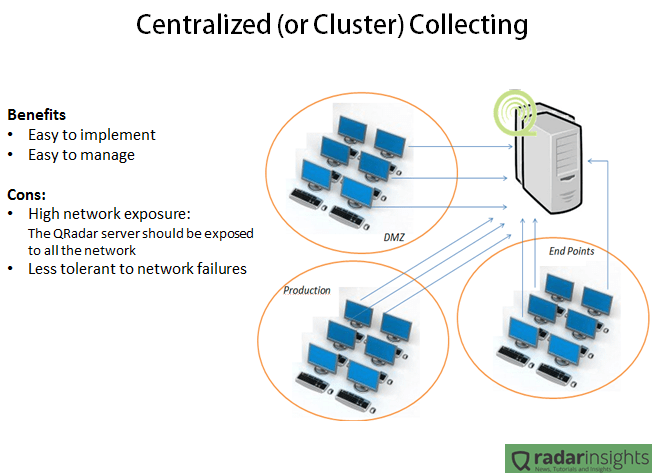
In the Centralized scenario, all the servers and collectors are in the same network. It makes the deployment and management way easier since we have just one point of maintenance and one point to “care about”, and it is very important especially when we have a geographically spread environment. But having all the SIEM solution in one network means that all the environment will need to connect to the cluster. In other words, the firewalls will allow traffic between the QRadar cluster and any server. Considering that some collection methods involves windows authentications, it means that if someone get access to the QRadar cluster network, the person will have access to any device on the network. Another bad point of this kind of deployment is the network failure tolerance. Lets say that the router in the border of the QRadar network goes down, all the log collection will be lost.

The distributed collection usually takes more time (and money) to implement and requires more time/resources to maintain, since the appliances will be distributed physically and logically. But the advantages are clear. With a distributed deployment the main QRadar console will have access only to its’ collectors, and nothing more. It means that if someone get access to the main SIEM network, the person will be able only to send packets to very specific IPs (collectors), and since the QRadar collectors are completely hardened, the security risk involved on this deployment is very low. Another benefit of the distributed deployment is the network failure tolerance. Considering the same case of a broken router in the QRadar console network, in this case the collectors will not have connection with the main console and will buffer the logs. After the network connectivity being restored, the logs will be synchronized with the main console.
As you guys noticed, the Distributed deployment can bring some good advantages compared with the Centralized one. But each company is a different case. Is up to you as an architect decide which deployment will fit your client need.
Do you have any suggestion or comment? Drop us a line in the comments!
Storage Sizing
In the last post we discussed how to calculate the EPS of our environment. Now lets discuss how to calculate the required size of the storage, since with the EPS in hands it turns way easier to calculate the size of our database. In this scenario we will consider only the log storage, not considering the network flows storage.
First of all, we need to understand how the data is stored on QRadar. Basically, you have 3 types of data:
- Online live data: All the events can be accessed with no latency. In this case the data is not compacted;
- Online compacted data: All the events can be accessed but with a small latency because the data is compacted. The avarage compression rate is 10:1;
- Offline data: All the events cannot be accessed instantly because all the data is in a external backup server. To access this data the user should import the backup into the QRadar (or into a QRadar Virtual Machine) for analysis;
After understanding which each type of data represents, we can start to calculate the storage based on the requirements of the project. In the sizing, we only use the Online data, the offline backup is not considered (since it is a external independent server).
To make an easy explanation, lets use the following requirements:
[Online Live Data: 7 days; Online Compacted: 180 days; EPS: 2500]
Steps to calculate:
- Calculate how much data is generated each second: Multiply the EPS by 300 bytes (the average size of an log):
In the example: 2500 x 300 = 750000 bytes = 732.5 kb/s - With the Data Per Second, we can calculate how much data we have in one day (1 day = 86400 seconds):
In the example: 732.5 * 86400 = 63288000 kb/day = 61804.7 Mb/day = 60.4 Gb/day - Now that we know how much data is generated in one day, lets calculate the Online Live Data size (non-compacted):
In the example: 60.4Gb/day * 7 = 422.8Gb - Now, lets calculate the Online Compacted Data. Note that the average compression rate is 10:1 :
In the example: 180 days – 7 days (online live data) = 173 days
173 days * 60.4Gb = 10449.2 Gb
10449.2Gb * 0,1 (compression rate) = 1044.92Gb - We have the size of the online live and the online compacted data. Now we just need to sum both and we have the final size:
In the example: 422.8Gb + 1044.92Gb = 1467.72Gb = 1.43Tb
Following this basic steps we can have a accurate approximation of the necessary storage size. A good practice is using a storage 20% bigger than the estimated.
Do you have any another experience with storage sizing? Let us know in the comments!
UPDATE: According to one of our readers (see comments), starting from the version 7.2.7, the stored data will always be compressed. So, if you are sizing your environment for the latest QRadar version, you should use only the “compressed data” calculations.
QRadar Sizing – Determining EPS
One of the biggest challenges when sizing a QRadar implementation is estimating the Events Per Second (aka. EPS) of the environment, specially because in the most of the cases we don’t have full access to the log sources to precisely determine the EPS. So in this post we will review some tips about how to estimate the EPS.
Determining the EPS of one event source with access to the system or access to the logfiles.
# Dump the log in a file and delete all the log not from the past 24h. Leave only the last 24h of logs
– If the system generate syslog, follow these steps:
a. Configure the logsource to send the logs to any linux server
b. In the destination linux server execute the following command: tcpdump -i eth0 src host SOURCE_IP dst port 514
c. Run the command for exactly 24 hours in a regular day and verify how many log packets you got.
# Verify the number of logs in the file.
– If there is just one log per line, simple open the file on notepad and verify how many lines you have;
– If the logs are not one per line, verify the whole size of the file (in bytes) and divide by 250 (the avarage size of a log line). Example: File with 3Mb = 3145728 bytes / 250 = 12583 Log packets
# Divide the number of packets by 86400, the result will be the EPS of the log source
Determining the EPS without access to logs or the system:
# From my previous experience, a good approximation of EPS is:
| Device Type | EPS |
| Active Directory | 15 |
| IIS or Exchange | 10 |
| General Windows Server | 2 |
| General Windows Workstation | 0,5 |
| UNIX/Linux Server | 0,5 |
| DNS or DHCP | 15 |
| AntiVirus Server | 20 |
| Database | 1 |
| Proxy | 25 |
| Core/Border Firewall | 150 |
| Small Firewall | 20 |
| IPS, IDS or DAM | 5 |
| VPN | 5 |
| Routers/Switches | 0,25 |
Calculating the EPS of the whole environment:
# Multiply the number of each device by the estimated EPS
# Sum the EPS of all kind of devices and you will have the EPS of your whole environment
– Example:
3 Core Routers + 2 IPS = 3x 150 + 2x 5 = 460 EPS
# Remember to always consider at least 20% margin for buying your license.
Do you have any another tips to calculate EPS? Let us know in the comments!
